Day 2
Introduction
In the previous session, we used some different data types produced by different technologies to reconstruct the full DNA complement of a target organism. Today, we will do some more work on the resulting genomes and try and assess how good our constructions are. We will use some concepts covered in the last session, such as k-mers, but we will also start to incorporate information about functional elements such as genes. Before we do that, it’s important to recap on what a genome contains, and how it functions.
The DNA sequence of an organism is sometimes referred to as the data storage structure of living organisms. This storage contains a dizzying variety of features: Their are sequences that can be transcribed into various species of RNA. Some of these RNA molecules can be active in their own right, such as micro-RNA or CRISPR sequences. Other transcribed sequences go on to be translated into strings of amino-acids, that ultimately produce functional proteins.
Figure 1. The central dogma of molecular biology
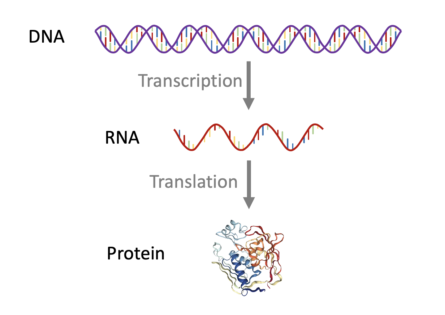
Many regions of DNA are not typically converted into other types of biomolecule, however they can still confer important structural properties (e.g. centromeres or telomeres), or provide regulation of the regions that are transcribed (e.g. promoters or enhancers). Genomes are also full of viral and non-viral mobile DNA sequences such as transposable elements, the differing activities of these mobile sequences are fascinating in their own right, and can have mutagenic activities, with important implications for evolutionary biology.
Genome annotation refers broadly to the identification of the various features in a genome sequence. Additional data is often used to achieve this. Rather than generate sequencing read data from genomic DNA, we can use the same technology to capture a sample of an organisms RNA. “Mapping” this data (aligning the RNA sequencing reads to a genome assembly), can provide evidence for the locations of transcribed sequence including their, start, end and gene splicing events. Based on the sequences within these annotations we can then predict resulting amino-acid sequences, and in some cases the three-dimensional structure of the resulting proteins.
Here is a genome browser displaying annotations for an E. coli reference genome, have a go at zooming in to see the various annotations on the genome, and then further to the nucleotide sequence:
5. Post-Assembly QC
Now that we have some assembled genomes from the previous session, we will explore them in some more detail. This should help you understand the strengths and weaknesses of the different data-types, and also how to assess different aspects of genome assembly quality.
Both Canu and Spades should have produced directories full of various files. Hifiasm should also produce output files, but for this program we need to do an additional step to generate a “fasta” file from the “gfa” file.
awk '/^S/{print ">"$2;print $3}' hifi_ecoli.p_ctg.gfa > hifi_ecoli.p_ctg.fa5.1. Assembly graphs and genome size.
We can visualise the assembly graphs for these three different datasets using the software Bandage. We use a specific file-type produced by some (but not all) genome assembly programs, known as a Graphical Fragment Assembly (.gfa) file. This format documents stretches of assembled sequence and also the relationship between contiguous runs, that may have multiple valid paths due to the presence of repetitive sequence or heterozygosity.
To use bandage in Window:
Use “scp” to copy the gfa or fastg files from the three assemblies to your local machine.
Download the program from this link https://github.com/rrwick/Bandage/releases/download/v0.8.1/Bandage_Windows_v0_8_1.zip
Open the zip archive and double click on the Bandage.exe file.
A window should open.
You can click File, then load graph, and you should be able to select a gfa file from one of your assemblies.
Click “Draw graph”
You can load bandage in Linux by:
typing the command “Bandage” into the unix command prompt.
A window should open.
You can click File, then load graph, and you should be able to select a gfa file from one of your assemblies.
Figure 3: A visualisation of the gfa file produced by Spades using the short Illumina read data. We can see that there is a tangle of valid paths, and also that the total length is higher than the size estimated from our earlier k-mer analysis. There are long stretches of contiguous sequence, which is useful genomic data, but the unresolved regions of the graph may inhibit some types of analysis. We would refer to this as a draft genome.
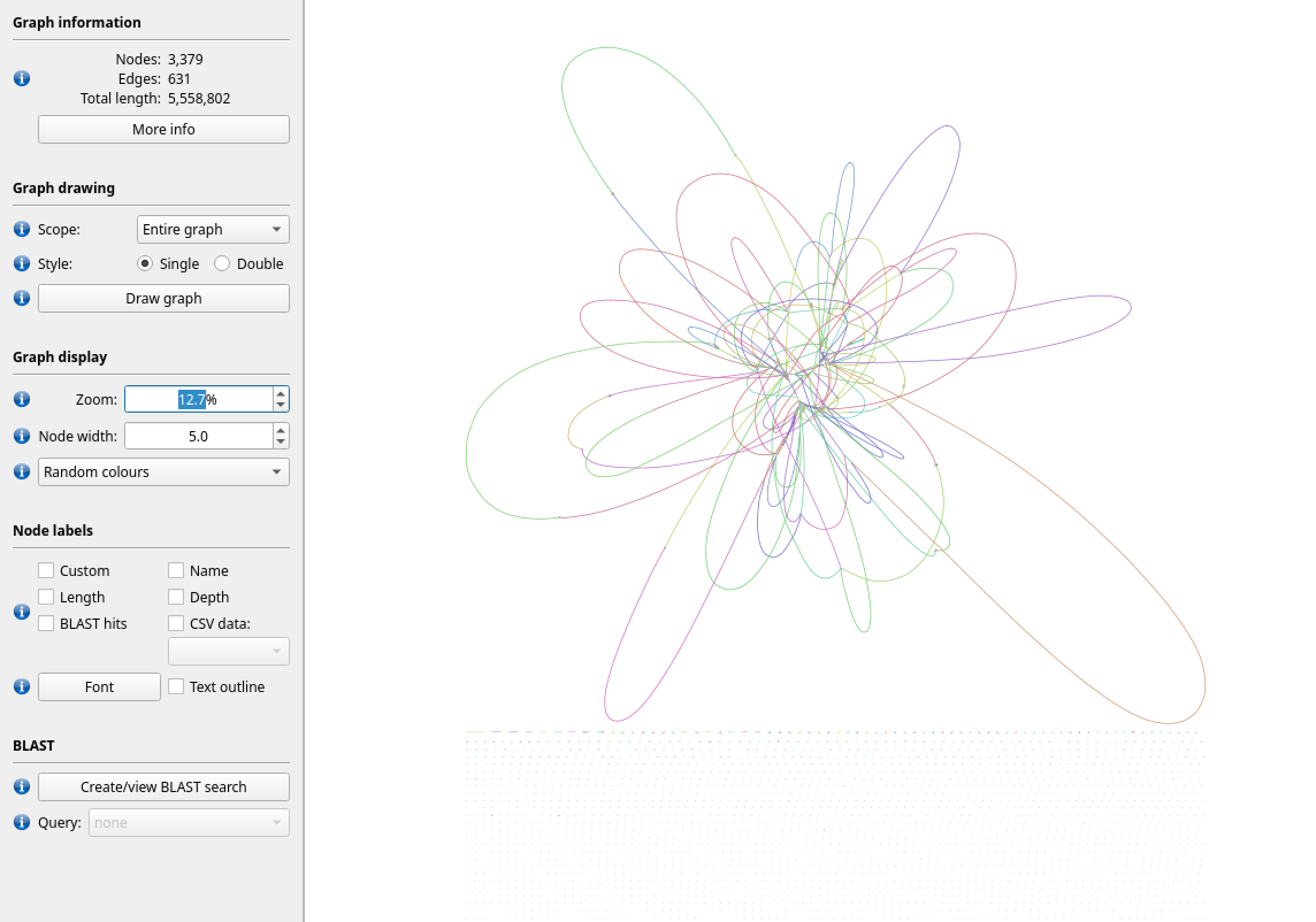
Figure 4: In contrast, here is a visualisation of the “unitig” gfa file produced by canu using the nanopore data. We can see that, for the most part there is a single clean path (node), and that the total length is roughly the size we expect. After checking the final contig sequence file (fasta), the loop structure is resolved into a single circular genome.
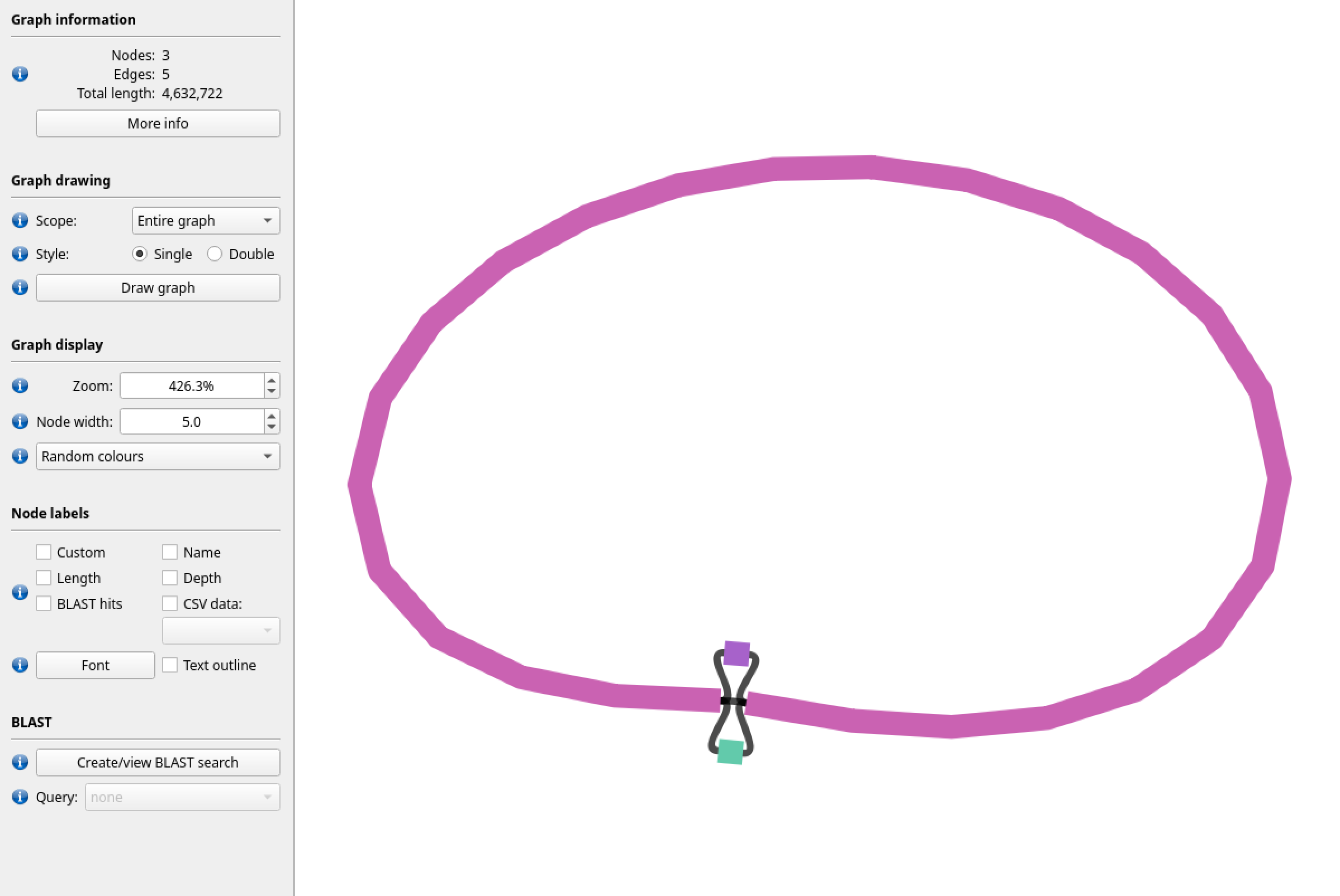
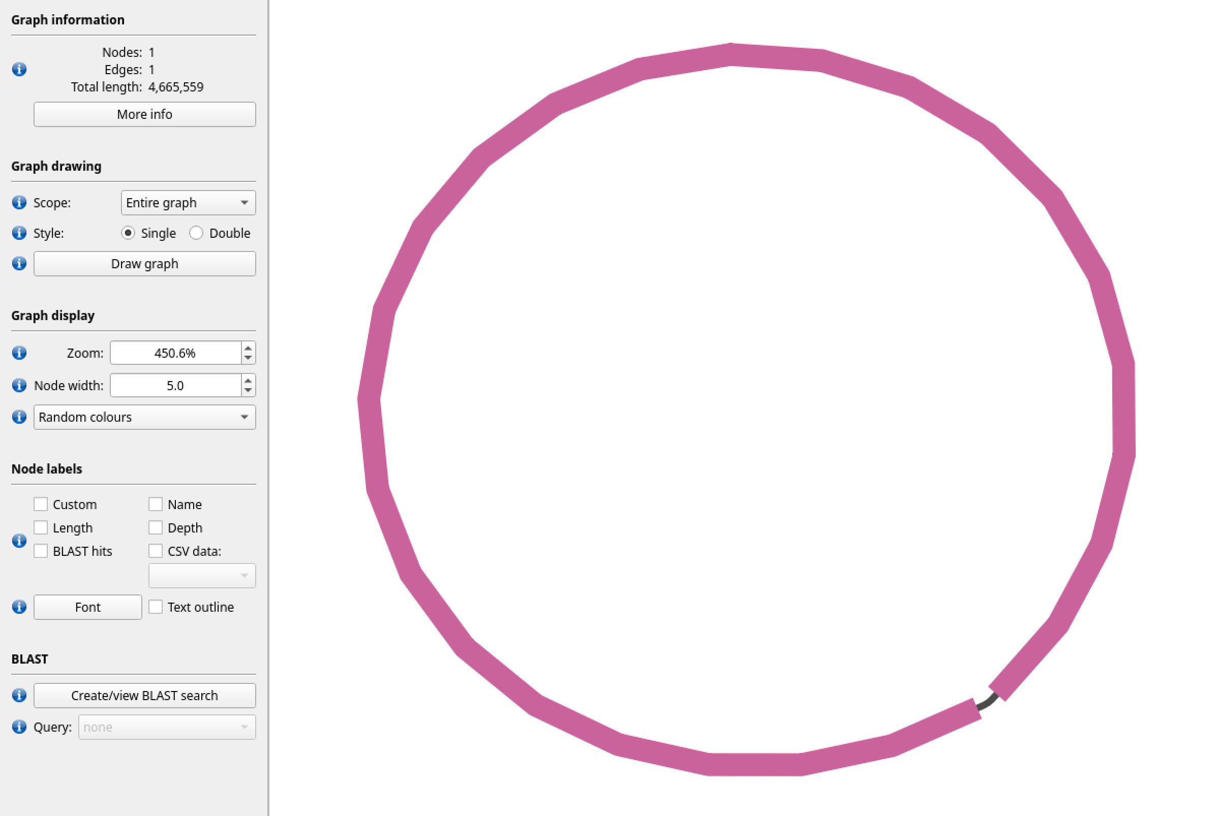
Figure 5: Here is a visualisation of the gfa file produced by hifiasm using the PacBio HiFi dataset. We can see that this data is able to resolve the genome into a single closed loop.
5.2. k-mer content
Another way to check the quality of a genome assembly, without having to rely on genes, is to compare the k-mer content that we saw in the raw reads to the k-mers present in the finished genome assembly. We can use the k-mer analysis toolkit to do this.
kat comp -t 16 -o SRR18106304_vs_spades SRR18106304.fastq ecoli_hiseq_spades/scaffolds.fasta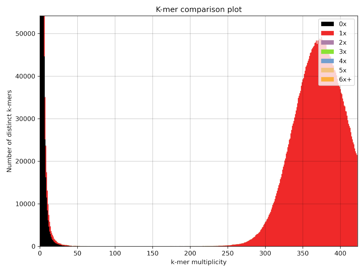
Here we can see the same distribution we observed earlier, however now we have colours added, which indicate how many times k-mers occur in the assembled genome. We can see here on the left hand side that many of the error k-mers are shown in black. This means the k-mers are not present in the assembly, which is good news. However, we can also see that some of these error k-mers are shown in red, which means there are some sequence errors still present in the draft assembly.
In comparison here is the same plot for the HiFi assembly.
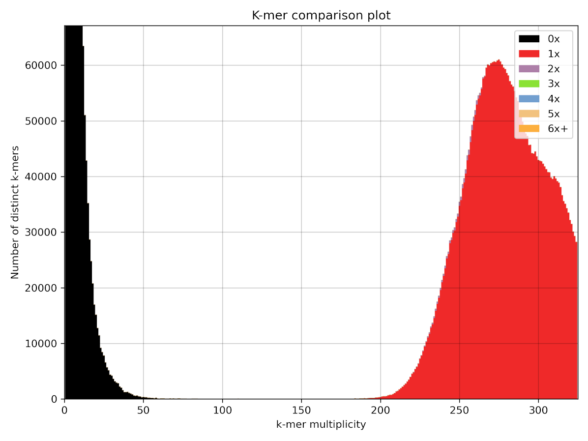
Now we can see that there are much less k-mers in the left hand peak present in the assembly. although we can see that a small number of k-mers in the right hand peak contains a small amount of purple duplicated k-mers!
5.2. Gene content
We can check the quality of an assembly, by checking whether “conserved” genes are present in our assemblies (see paper for details). Using the software BUSCO (Benchmarking Universal Single-Copy Orthologs), we can generate some information about whether genes are present or absent, fragmented across contigs, or whether they’re present in the right number.
Here we are performing a specific type of genome annotation, which attempts to identify a specific set of conserved genes, that are often only present in a single copy. If some of these genes are missing, it provides some evidence that our genome assembly may not be complete. Alternatively if these genes are found more than once, it provides some evidence that our assembly may have incorrectly duplicated some genomic regions.
##Bash/command line code
busco -m genome -i /scratch/ecoli_hiseq_spades/scaffolds.fasta -o Hiseq_busco --auto-lineage-prok
Have a browse through the output files in the output folder Hiseq_busco and see if you can find out how complete this genome assembly is. You can also generate an analysis for the other genomes you assembled yesterday (make sure to change the name of the output file!) and compare the results.
5.4. Quast report
Before we move on to some other checks we are going to run the program quast, which performs a range of checks for you. We can run this as indicated below. For the purposes of demonstration we will use a reference genome to check our data against, but for a novel genome assembly we would not have this data.
We are going to run this software with another form of annotation, to help us assess the quality of our genome assemblies. The Glimmer method is specifically designed to detect prokaryotic genes, without the need for additional data.
First find an E. coli k-12 reference genome on NCBI (https://www.ncbi.nlm.nih.gov/), as shown below.
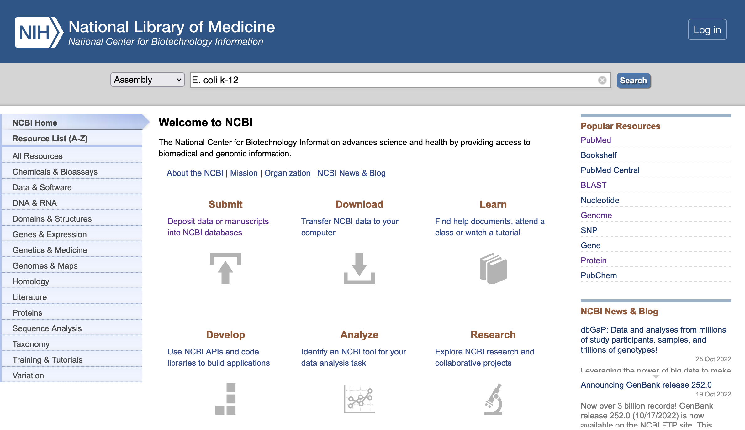
Select one of the resulting genome assemblies.
Now click on the link on the right hand side of the page labelled “FTP directory for RefSeq assembly”
Here you can see a range of information including the genomic sequence files annotations and other associated statistics.
Right click on the file that looks like this “GCF_905147045.1_ilAglIoxx1.1_genomic.fna.gz” and copy the link.
Now in your Unix terminal navigate to your home directory and paste the link after a “wget command”, in the same format as below (make sure to paste in the correct link that you’ve copied).
wget https://ftp.ncbi.nlm.nih.gov/genomes/all/GCF/000/005/845/GCF_example/GCF_example_genomic.fna.gz
Now you are ready to run quast with your three previously assembled genomes.
Load both modules for quast
module load anaconda2/4.2.0
module load quast/4.6.0
quast.py -R GCF_000005845.2_ASM584v2_genomic.fna --glimmer --output-dir test_quast ./Hifi_ecoli.fa ./ecoli-oxford/ecoli.contigs.fasta ./ecoli_hiseq_spades/scaffolds.fasta Have a look at the quast report by loading the html file.
firefox test_quast/report.html
6. More complex genomes
So far we have only considered a haploid bacterial genome, with a very small overall size. In such simple genomes an assembly graphs may suggest multiple paths through a given sequence due to repeating sequence, but we know that there is likely only one biologically real path through the graph. In diploid (and polyploid) organisms, this becomes more complicated because there are more than one real biological paths through the graph. These alternate paths are due to the presence of sister chromatids, that are not identical to each other, due to the presence of genetic variation, or heterozygosity. A key factor in assembling high quality genome assemblies, is the “phasing” of the chromosomes. It can be difficult to distinguish whether a given heterozygous region belongs to one chromosome copy or the other. Variation found on the same chromosome copy is in “linkage” or can be said to have the same “phase”. A perfect genome assembly would reconstruct the variation from each chromosome perfectly as found in the original organism, however in practice this can be difficult to achieve. The figures below should help to explain this problem and explain potential solutions.
Figure 6: A common result from sequencing diploid genomes is the presence of redundant haplotypes in the final assembly, particularly for regions with have a high sequence divergence. Here we can see homozygous regions in orange, and a reconstructed reference contig which contains a mosaic of haplotypes from two different sister chromatids (indicated in yellow and blue).
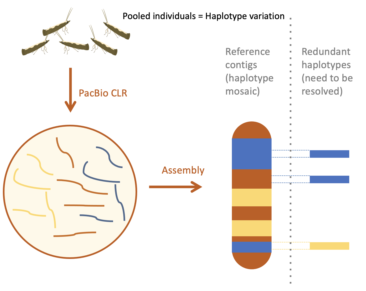
Figure 7: One method of resolving heterozygosity in a genome sequencing project is to gather parental data and use this to partition the chromatids inherited by the F1 offspring. In this example, we generated long reads for an F1 individual and short Illumina reads for the parents. We were able to use the Illumina reads to separate the F1 PacBio reads into two groups for assembly.
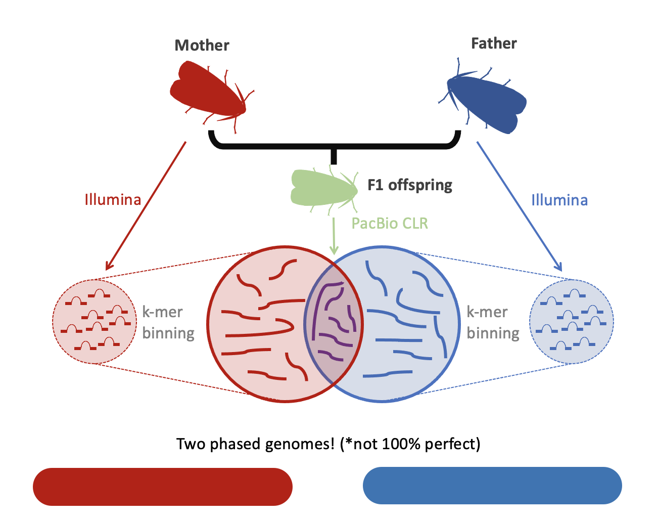
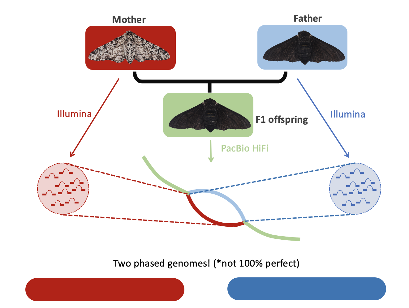
Figure 7: Another way to utilise parental data is to use the k-mers during the construction of the assembly graph itself. Specifically, we can identify bubble structures that are likely to represent heterozygous regions and look for parent specific k-mers in the alternate paths. Crucially, this approach requires high accuracy long reads such as HiFi data to work successfully.
7. Genome alignment
We are going to download some datasets, you may choose two species from the following list to align:
| Name (common) | NCBI RefSeq accession |
|---|---|
| Melitaea cinxia (Glanville fritillary) | GCF_905220565.1 |
| Pararge aegeria (specked wood butterfly) | GCF_905163445.1 |
| Nymphalis io (European peacock) | GCF_905147045.1 |
| Vanessa cardui (painted lady) | GCF_905220365.1 |
| Leptidea sinapis (wood white) | GCF_905404315.1 |
| Maniola jurtina (meadow brown) | GCF_905333055.1 |
| Vanessa atalanta (red admiral) | GCF_905147765.1 |
| Plutella xylostella (diamondback moth) | GCF_932276165.1 |
| Pieris rapae (cabbage white) | GCF_905147795.1 |
| Pieris brassicae (large cabbage white) | GCF_905147105.1 |
| Colias croceus (clouded yellow) | GCF_905220415.1 |
| Papilio machaon (common yellow swallowtail) | GCF_912999745.1 |
| Pieris napi (green-veined white) | GCF_905475465.1 |
| Aricia agestis (brown argus) | GCF_905147365.1 |
In section 5.4 we downloaded an E. coli reference genome. You will need to perform this same process for each of your chosen species.
Once you have the genomic fasta files downloaded, we can try out a pairwise genomic alignment between two of your species. We’ll use the tool minimap2, which was designed to map long sequences to a genome, such as pacbio reads, however using specific parameters we can also use it to perform alignments between species that are not too distantly related (i.e. within the same Family, or Order).
Using two fasta files we can compute a “paf” alignment file (here I use Aricia agestis and Vanessa cardui), like so:
~/bin/minimap2/minimap2 -PD -x asm5 -t 16 GCF_905147365.1_ilAriAges1.1_genomic.fna GCF_905220365.1_ilVanCard2.1_genomic.fna > AriAges_VanCard.pafWe can then use an R script to convert this alignment into a dotplot style figure. This type of figure represents a query genome on one axis and a target genome on the other axis. Dots correspond to matches between the two sets of sequences. Some dots will appear across many different chromosomes, these matches are likely to correspond to repetitive sequences such as transposable elements. Other matches form intermittent diagonal lines, and are likely to represent orthologous regions of the genome. When the angles of these diagonal lines change direction, they may represent “inversion” polymorphisms. This type of polymorphism occurs, when a large section of a chromosome flips-over (inverts), due to a breakage and erroneous repair.
Rscript ~/Workshop_materials/pafCoordsDotPlotly.R -i ColCroc_AriAges.paf -o ColCroc_AriAges.out -s -t -m 1500 -q 5000008. RNA-seq gene annotation
Earlier, we used some different annotation methods to model some genes found in a simple bacterial genome. Now we are going to have a go at using additional data to find genes in a more complicated organism. We will be using a very recent high quality genome for the diamondback moth.
8.1. Data download
First let’s download the genome data:
wget https://ftp.ncbi.nlm.nih.gov/genomes/all/GCF/932/276/165/GCF_932276165.1_ilPluXylo3.1/GCF_932276165.1_ilPluXylo3.1_genomic.fna.gzand also some RNA seq data (It is pre-downloaded in /home/taller-2019/Workshop_materials/). The tissue that RNA is sampled from is very important. RNA composition varies very dramatically between tissues, developmental stages and environmental conditions. This sample comes from an adult moth, and therefore may not contain genes that are very specific to other stages, such as ovum, caterpillar & pupae.
fasterq-dump SRR150425368.2. Mapping
Now in order to map the RNA-seq reads, we first need to index our genome.
First, decompress the genome:
gunzip GCF_932276165.1_ilPluXylo3.1_genomic.fna.gzThen index like so:
hisat2-build GCF_932276165.1_ilPluXylo3.1_genomic.fna GCF_932276165.1_ilPluXylo3.1_genomic_hisat2_indexAfter a few minutes, we should have our genome indexed and ready for mapping. We can map our RNA-seq reads like this:
hisat2 -S SRR15042536.sam -p 10 --rna-strandness=FR -x GCF_932276165.1_ilPluXylo3.1_genomic_hisat2_index -1 SRR15042536_1.fastq -2 SRR15042536_2.fastqNow we need to sort the resulting file and convert it to a compressed bam format (SAM is the human-readable version). We can also index the resulting bam, for visualisation purposes.
samtools sort -o SRR15042536.sorted.bam SRR15042536.sam
samtools index SRR15042536.sorted.bam
8.3. Transcript assembly
Now that we have our mapped reads, we can use the information to produce some gene models.
stringtie -o SRR15042536.gff SRR15042536.sorted.bamYou can now have a look at the annotation you’ve produced as well as the mapped read and see how the program is able to use RNA alignment evidence to build gene models.
IGV may not run on Kabre, but you can install it on your local machine (here), or try the web app (here):
For the web app you first need to generate an index file using the samtools program, like this:
samtools faidx example_genome.faYou then need to download both the .fa and the .fai (produced by the previous command) to your local computer. To load this genome in the web app, you must select both files when loading the genome.
This should open a new GUI window. First load your genome, by clicking Genomes -> Load Genome From File. Then you can load the sorted.bam file and the gff, by clicking File -> Load from file.
9. Homology gene annotation
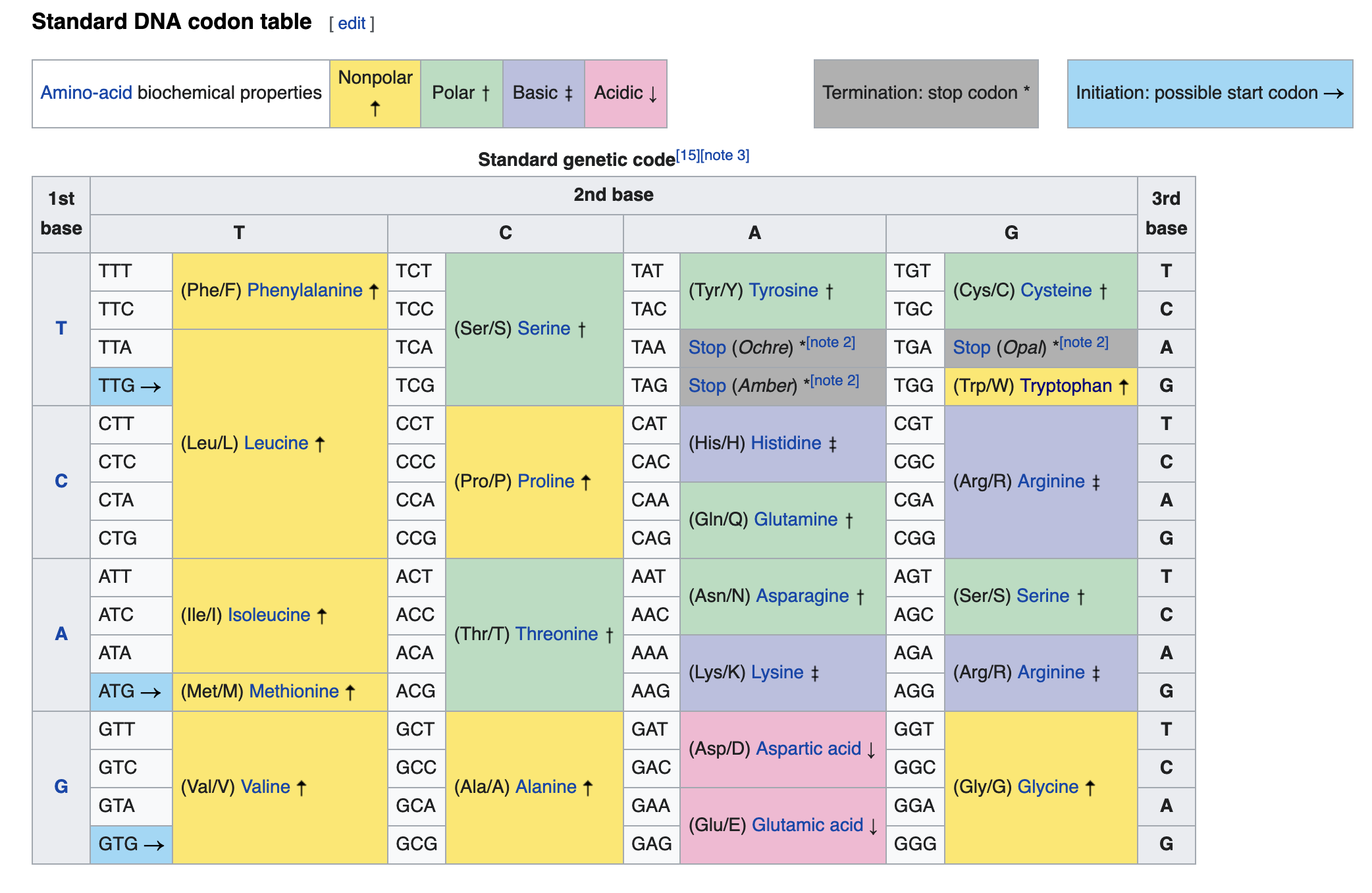
An alternative way to infer the presence of a gene is to use amino-acid sequences from closely related organisms. For many important protein sequences, purifying selection eliminates mutations that alter the amino-acid sequence, however coding sequences are still able to accumulate mutations in certain positions due to the fact that more multiple codon sequences are able to code for the same amino-acid.
We will align some proteins for a very fast evolving gene and see how they compare to the RNA-seq data you’ve mapped. Here’ we’ll take a selection of the same protein from different organisms and see how their different levels of evolutionary divergence interferes with the alignment process.
Aligning proteins with miniprot is very simple, the minimal command is:
miniprot -t8 --gff GCF_932276165.1_ilPluXylo3.1_genomic.fna Masc_multiSpecies_aa.fasta > prot1.gffWe can also tweak some of the parameters, and see how it affects the alignment:
miniprot -n 3 -s 3 -k 5 -l 3 -j 1 -t8 --gff GCF_932276165.1_ilPluXylo3.1_genomic.fna Masc_multiSpecies_aa.fasta > prot2.gff10. Homology gene clustering
The determination of shared ancestry between genes in divergent species is a complex process. Reproductive isolation and other processes lead to varying levels of sequence divergence along different branches of an evolutionary tree. Genes may also become duplicated or rearranged, gain or lose specific functions. Interestingly, the evolutionary history of individual genes, may be radically different from a species tree, due to processes such as Incomplete lineage sorting, trans-species polymorphism (e.g. via balancing selection) and molecular convergence (see here). Thus, we may need to compare the trees of many genes to assess the true evolutionary tree of the species themselves.
A useful program orthofinder, provides many of these functions in an automated tool. Let’s download some protein data for five of the butterfly species in the table above (more species will take more time to run).
First make a new directory called orthofinder_1 and move into that folder.
mkdir orthofinder_1
cd orthofinder_1
Then, navigate to the FTP site for each species using the links above, then right click and copy the link to the “_protein.faa.gz” files. Use the wget command to copy the data into the new folder like so:
wget https://ftp.ncbi.nlm.nih.gov/genomes/all/GCF/905/220/565/GCF_905220565.1_ilMelCinx1.1/GCF_905220565.1_ilMelCinx1.1_protein.faa.gzDecompress the protein files like this:
GCF_905220565.1_ilMelCinx1.1_protein.faa.gzOnce all the files are decompressed, you can run orthofinder like this:
orthofinder -f ~/orthofinder_1This might take a little bit of time (there is a pre-computed output folder in the /home/taller-2019/Workshop_materials/ folder), but once complete, it is worth looking through the resulting output files (see here). In particular you should now have a resolved species tree, and also trees for all genes in the inferred orthogroups. A simple way of viewing this data is to paste it into this website.